Roots of Unity
The n-th roots of unity are evenly spaced points on a circle. Under multiplication, they work together as one cyclic group.
An interactive atlas of number theory
Begin with points on a circle, then discover the arithmetic that brings their patterns to life.
At first, a Gaussian period looks like a simple sum of points on the unit circle. But when those points are chosen according to a pattern in modular arithmetic, the sum begins to reveal a deeper structure connecting algebra, number theory, and geometry.
The construction begins with powers of a primitive n-th root of unity. We group their exponents using a multiplicative subgroup or one of its cosets, then add the corresponding roots. Each part is familiar on its own; together, they produce the algebraic numbers known as Gaussian periods.
The exponents in one multiplicative coset select the roots that are added to form a Gaussian period.
The n-th roots of unity are evenly spaced points on a circle. Under multiplication, they work together as one cyclic group.
Multiplicative cosets sort the exponents into distinct groups. Characters give us another way to recognize those same groups.
A period and its Galois conjugates fit into one monic polynomial, giving us an exact record of the period's algebraic structure.
The n-th roots of unity sit at equal intervals on the unit circle. For n=12, the twelve points form a regular 12-gon, turning the equation z12=1 into a shape we can see.
Next, we repeatedly multiply the exponents by a unit ω modulo n. This sorts the roots into multiplicative orbits. Adding the roots in each orbit turns separate points into the cyclotomic sums that underlie Gaussian periods.
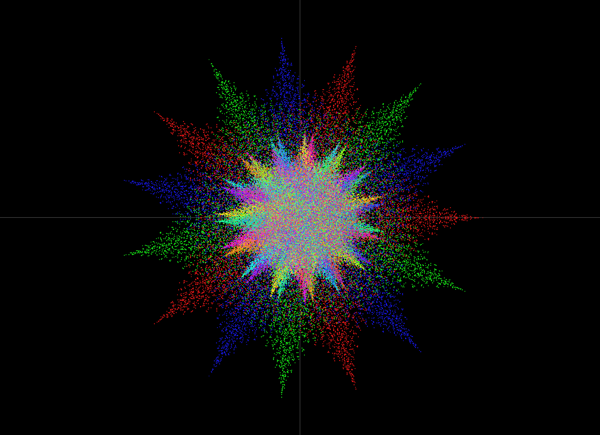
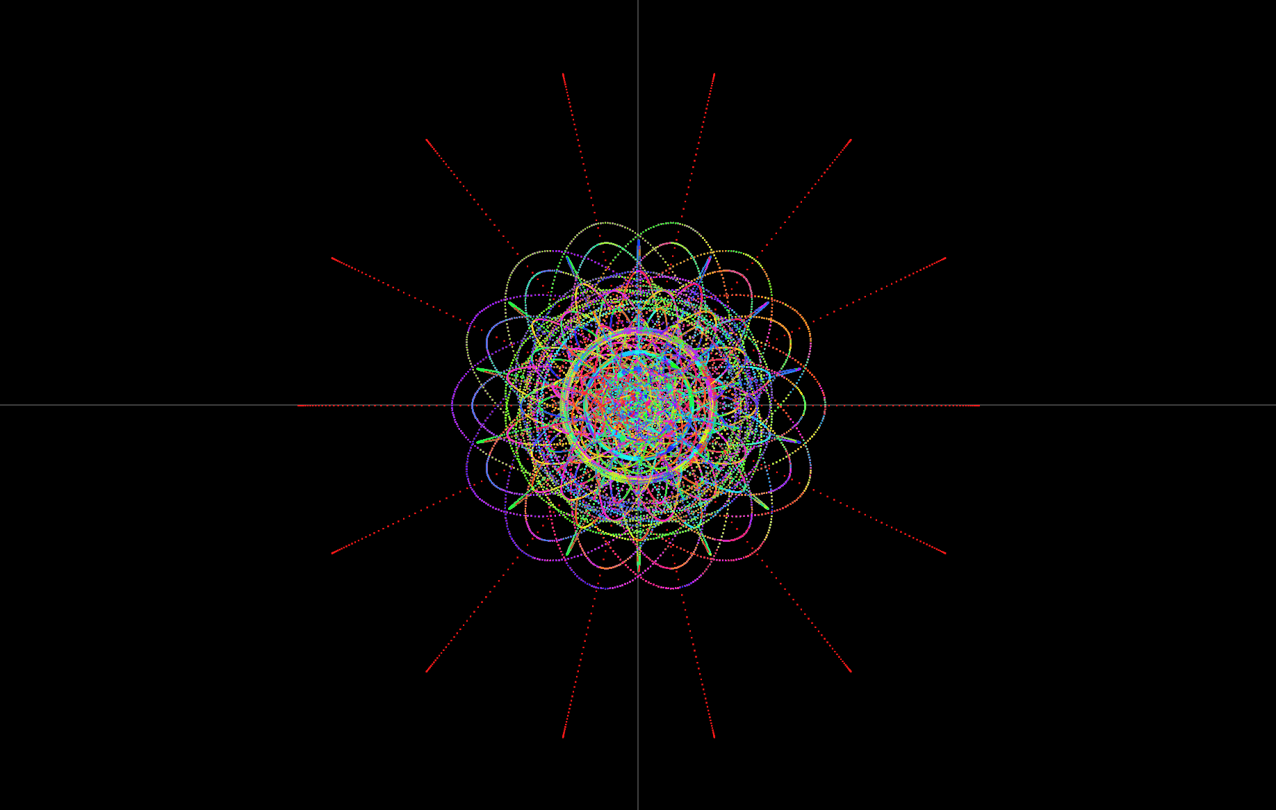
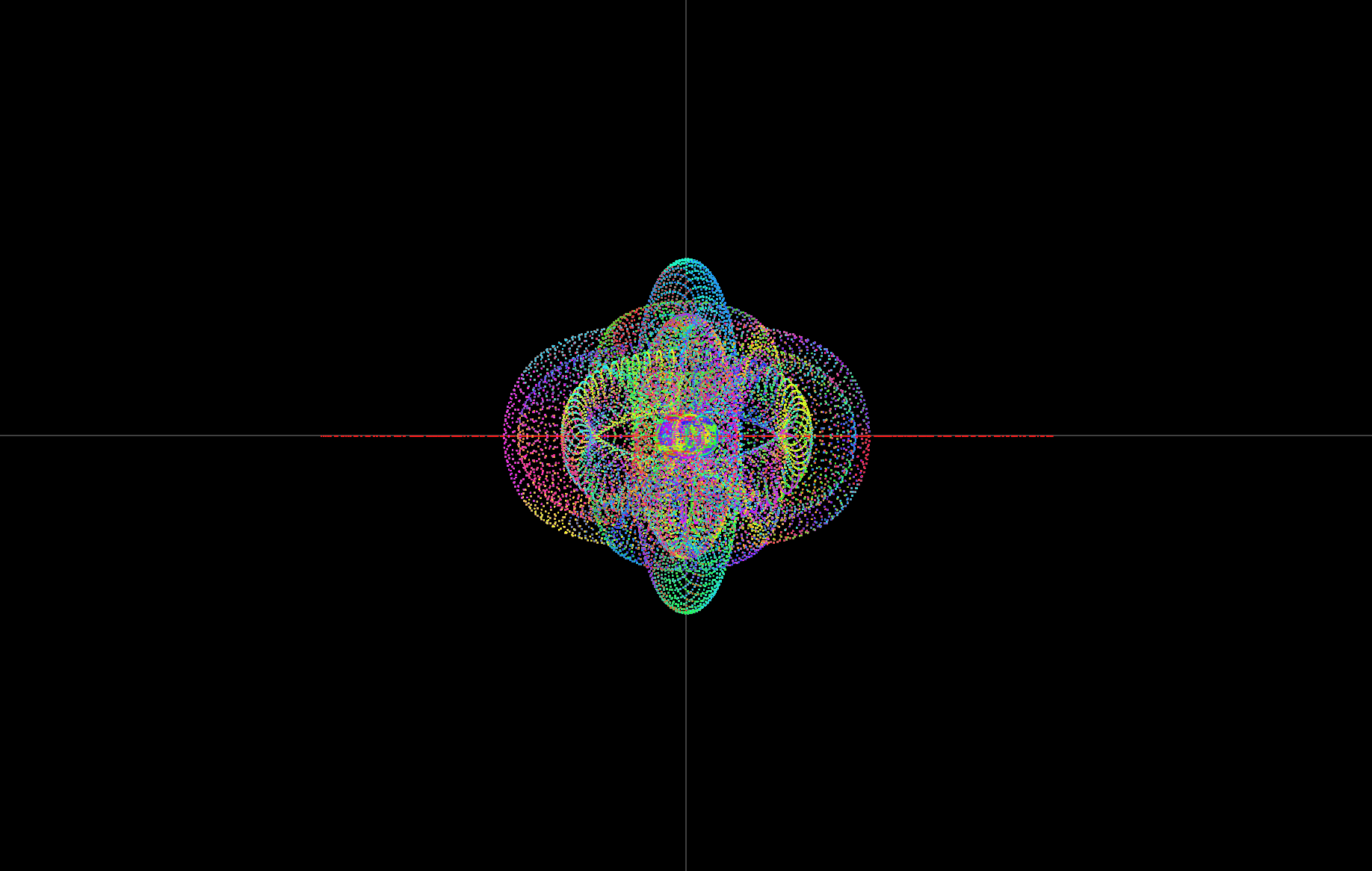
Each plotted point has a calculation behind it. Follow the roots as they are selected, added, and placed on the complex plane:
The coloring begins with the exponents. A parameter ω repeatedly multiplies them modulo n, placing exponents that follow the same cycle into one orbit. Each orbit then selects a group of roots of unity, and adding those roots produces its Gaussian-period sum:
Each root ζnj = e2πij/n has a real and an imaginary component. Their sum, ηk, does too. The visualizer places that sum on the complex plane, with its real part on the x-axis and its imaginary part on the y-axis.
Once the points are computed, modular arithmetic assigns a color to each index k:
Here, c is the number of colors, so the result always lies between 0 and c−1. With c=3, points 0, 1, and 2 receive three different colors before point 3 returns to the first. As the cycle repeats, the colors make the underlying order easier to follow.
This example follows the 12th roots of unity from separate points to grouped and colored orbits:
First, all twelve roots appear on the unit circle. Then multiplication by ω=7 separates them into equivalence classes. Finally, the roots are grouped and colored by period, allowing the structure to emerge one step at a time.